What the system has found.

Discovery does not need a data centre. All 112 results here came from two small cloud machines.

Combinatorial designs

Hadamard matrices, difference sets and weighing matrices are perfectly balanced arrangements. They sit underneath error-correcting codes, radar and the design of experiments, and for most sizes nobody knows whether one exists.

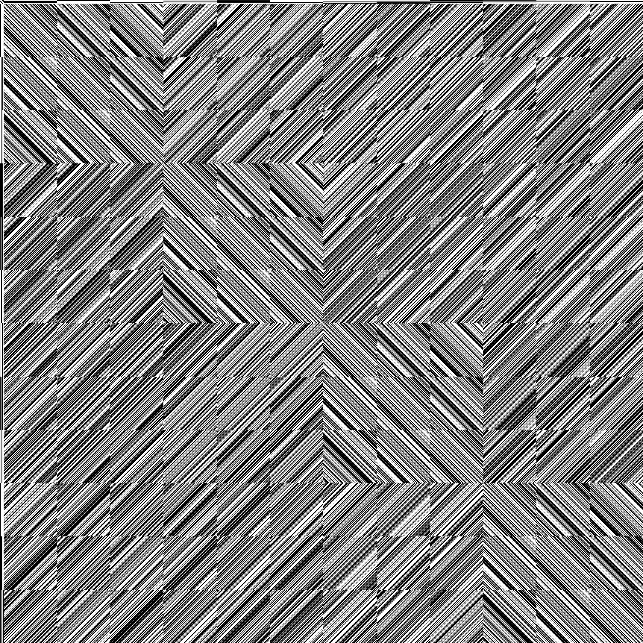
Part of our Hadamard matrix of order 2148, at two pixels an entry.
Difference sets

No cyclic relative difference set with kernel order above 1 lifts a difference set with parameters (364, 121, 40), (255, 127, 63), (1464, 133, 12) or (2380, 183, 14).

Gordon (2026) lists the 4 as open, except kernel order 2 for (364, 121, 40), settled by search; his Theorem 5 excludes kernel order 7 for (2380, 183, 14) as printed. Only that case can be checked from published files.

Weighing matrices

CW(180, 36) has 12 inequivalent proper matrices, and an exhaustive computation of ours finds no further one and no circulant weighing matrix at 12 other parameter pairs.

CW(180, 36) and the 12 pairs were listed “Open” in La Jolla version 1.3. Gordon announced 4 of the 12 non-existence results, which we cede, and an unnamed existence result, which may be this one, on 19 October 2026.

Weighing matrices

Of 2,763 covered pairs listed “Open” in La Jolla version 1.3, we recorded 2,397 as decided: 2,342 with no matrix, 25 with a proper matrix, 30 with improper matrices only.

Counts are as of 26 October 2026. We treat CW(182, 144) and CW(155, 100) as unresolved, leaving 2,395 decided. Version 2.0 lists 115 of the non-existence results as “No”; we claim no priority.

Hadamard family

For every prime power q ≡ 3 (mod 4) there is a skew-Hadamard matrix of order 3(q + 1), and three further constructions give symmetric Hadamard matrices.

With the accompanying searches, these settle 106 skew and 85 symmetric values that the 2025 census of Đoković and Seberry lists as undecided.

Hadamard family

An exhaustive computer search finds exactly one inequivalent set of circulant Williamson matrices of order 75, of Turyn type.

Turyn (1972) constructed order-75 Williamson matrices; Lang and Schneider (2011) reportedly print a Turyn-type set. If they list all such sets, the search adds only that no other type exists. One program of ours made the search, without a certificate.

Hadamard family

An exhaustive computer search finds no circulant good matrices of order 75.

The search covers the 4,898,576 instances, in the sense of Bright et al. (2019); we know of no published count at order 75. One program of ours made the search, without a certificate.

Hadamard family

Circulant good matrices of orders 53 and 55 exist; we give one explicit set of each.

To our knowledge no earlier good matrices of order 53 or 55 are published. The skew-Hadamard matrices of orders 212 and 220 they give were already known.

Hadamard family

Our complete searches at orders 59 and 65 find no circulant good matrices.

Published classifications of good matrices reach order 49 and, at multiples of 3, order 69.

Method

We reproduce all 44 published Williamson and good-matrix counts at odd multiples of 3, 9 to 69, and complete instances 1,100 to 5,000 times faster than the authors’ SAT step.

300 sampled instances, one core, Williamson orders 45 to 63, authors’ code ported to Python 3; ratios from an earlier build vary between repeats. Whole runs took 3,100 to 47,000 times less CPU time than printed hours, from older hardware.

Integer sequences

The OEIS records the numbers mathematicians have managed to compute. A sequence usually stops at the point where the next term was out of reach.

One complete mapping of Z31.
2,427,915,096,775,283,929,115
a(15): complete mappings of Z31 fixing 0
Complete mappings

We computed a(13), a(14) and a(15) of OEIS A003111, the numbers of complete mappings of Z27, Z29 and Z31 that fix 0; a(15) is 2,427,915,096,775,283,929,115.

In November 2026, A003111 listed terms to a(12), the order-25 term credited to Yuh-Pyng Shieh (2006). To our knowledge no source lists these 3 values.

Complete mappings

We counted the complete mappings of 23 groups: 21 of orders 24 to 28 and 2 of order 32.

Wanless (2007) gives counts for orders 3 to 23 and Z25, and ours agree for orders 3 to 23. The other 6 of orders 24 to 28 have none (Hall and Paige). To our knowledge no source lists these counts.

Self-dual codes

We computed the number of binary self-dual codes of each even length from 42 to 56, up to coordinate permutation.

In November 2026, OEIS A003179 listed lengths up to 36. Totals are published for lengths 38 and 40; to our knowledge none is published for length 42 or above.

Stabilizer states

We computed 8 terms of OEIS A094927, the number of stabilizer states on 13 to 20 qubits up to equivalence, and derived the matching terms of A090899.

In November 2026 both sequences listed terms to 12 qubits. Danielsen and Parker (2006) gave a lower bound of 72,573,549 for 13 qubits; we find 99,941,357.

Coding theory and telecom

A code’s minimum distance decides how many errors it can survive. Computing it exactly is NP-hard, so standards and tables often list a bound where the true value is unknown.

5G NR

We computed the minimum distance of 860 sub-codes of the 5G NR base graphs, each with an explicit codeword of that weight.

Each takes the first rows of base graph 1 or 2 at one lifting size, some punctured; lengths reach 11,904. These are sub-codes, not the standard’s full codes. We claim no priority over the KAIST CoCoA Lab database of codewords.

Linear codes

Five binary linear codes, [111, 37, 27], [152, 38, 42], [172, 43, 46], [159, 53, 35] and [174, 58, 37], have minimum distance above the lower bounds listed at codetables.de.

Each exceeds the lower bound listed in November 2026, by 1 for 4 codes and by 2 for [152, 38, 42]. Novelty is not established. These five and codes derived from them raise the lower bound in 24 cells.

Quantum error correction

A quantum memory survives only if no small set of faults can corrupt it. Circuit distance is the size of the smallest such set in the circuit that actually runs the code.

IBM’s two-gross code on its torus.
Bivariate-bicycle codes

Our rebuild of the Bravyi et al. two-gross [[288, 12, 18]] memory circuit, 18 noisy cycles, has circuit distance exactly 16 in both bases, below the published upper bound 18.

Crocker posted 16-fault sets in October 2026. Cheng, Guo and Pan (November 2026) are the earliest public report we found of the exact value, certified. Our lower bound is an unreleased computation; we claim no priority for the upper bound.

Bivariate-bicycle codes

G. Pan’s period-11 gross-code schedule, applied to the [[288, 12, 18]] code, has circuit distance 18 in both bases for 1 to 40 noisy cycles.

Pan’s repository gives no result for this code. The lower bound is an unreleased computation of ours, in our circuit builder’s noise model. For 41 to 45 cycles the value follows from a time-shift identity; beyond 45 it is assumed.

Bivariate-bicycle codes

Two non-interleaved schedules of ours, C1 and C2, give [[288, 12, 18]] memory circuits of circuit distance 18 in both bases, in the noise model of Strikis, Browne and Beverland.

Cheng, Guo and Pan (November 2026) are the earliest public report we found of schedules reaching 18 for this code; we claim no priority. The extended-code distance 18 is an unreleased computation of ours; the reduction is not re-proved here.

Bivariate-bicycle codes

The X-basis memory circuit of the [[360, 12, 24]] code in tesseract-decoder’s test data, 24 rounds, SI1000 noise, has circuit distance at least 19.

dist-m4ri’s benchmark file (commit e9cac19, 5 November 2026) lists 12 to 23 for this circuit. Weights up to 18 are excluded by an unreleased computation of ours. We know of no circuit-level result for this code published by IBM.

Syndrome cycles

We find 196 period-8 translation-invariant syndrome cycles of the [[108, 8, 10]] bivariate-bicycle code with circuit distance 10 in memory experiments of 4 noisy rounds (13 for 153 of them) started at each basis's cut.

IBM's depth-8 cycle has distance 8 (Kornstein); G. Pan posted distance-10 circuits for this code, among them a translation-invariant period-11 one. Of the 664 period-8 translation-invariant cycles with a cut per basis and extended distance at least 8, 196 reach distance 10. A further 1,208 cycles with a cut per basis were mostly not examined, so 196 does not count the class.

Logical error rate

Under SD6 noise and BP-OSD, a period-8 [[108, 8, 10]] cycle with circuit distance 10 has 0.76 [0.68, 0.86] times IBM's per-round logical error rate at p = 2.5×10⁻³; direct sampling resolves no benefit from 3×10⁻³ to 5×10⁻³.

Ten rounds, perfect preparation and readout, both bases added. Two pipelines pooled at 2.5×10⁻³ (4.4 standard deviations); one pipeline at 3×10⁻³ and 5×10⁻³ gives 0.90 [0.70, 1.16] and 1.08 [0.89, 1.30]. Fault-count stratified estimate at 3×10⁻³, with decoder priors there, is 0.77 [0.68, 0.88]; a benefit there is not excluded. Relay-BP-1 (4×10⁻³, 5×10⁻³) and SI1000-style noise (2.5×10⁻³) show no detectable gain. G. Pan reported no gain at p ≥ 10-3 for a non-uniform two-colour circuit.

Fault locations

A period-P single-ancilla CNOT cycle of an n-qubit bivariate-bicycle code, with every data qubit in three X and three Z checks and separate reset and measurement, has n(P + 2) SD6 fault locations plus one per idle ancilla step.

At period 8 every gross-code cycle in which no qubit is in two operations in a step and each ancilla's operations fit in one period has 1440 locations, IBM's count, and each further tick adds at least 10% of it; reset-free and fused ancillas are outside the statement. Strikis, Browne and Beverland gave the depth bound and idle counts; we know of no earlier closed count.

Gross-code cycles

Every gross-code [[144, 12, 12]] cycle evaluated in the classes searched, including all 22,608 uniform period-8 cycles, at 0.9 to 1.4 times IBM's fault locations, has circuit distance at most 11 in long enough memory experiments.

Also searched: 416,496 two-coloured period-8 cycles of the seven top hook-order classes with one colouring for X and Z; 8,784 uniform period-7 cycles with fused measurement and reset (0.9 times IBM's locations); compact-window uniform cycles of the top hook-order classes at periods 9 to 12 (1.1 to 1.4 times; at period 12, 8,864 of 10,432, one per class of equal fault sets). Strikis, Browne and Beverland proved the bound 11 for non-interleaved cycles.

Distance 11

Under SD6 noise and BP-OSD, a uniform period-8 gross-code cycle with circuit distance 11 and IBM's fault count has 1.04 [0.90, 1.20] times IBM's per-round logical error rate at p = 4×10⁻³, no detectable gain over distance 10.

Both values pool two pipelines over 12 rounds in both bases; at p = 5×10⁻³ the ratio is 1.05 [0.93, 1.18]. The cycle is G. Pan's, and ours is the same with all times shifted by one step. Cheng, Guo and Pan reported a tie within statistical error for an eight-timestep distance-11 schedule.

Decoding

On identical fault sets of IBM's gross-code cycle under SD6 noise, Relay-BP-1 has 0.24 [0.09, 0.55], 0.26 [0.12, 0.50] and 0.41 [0.25, 0.65] times the failure fraction of BP-OSD at 44, 52 and 60 fired mechanisms.

Z memory, 12 rounds, decoder priors at 3×10⁻³; Relay-BP-5 has 0.21 [0.12, 0.33] at 60, pooled over two samples, and 0.37 [0.20, 0.62] in the second alone. Müller et al. report Relay-BP-5 about one order of magnitude below BP+OSD at 3×10⁻³. Our ratios are failure fractions at fixed fault count, not per-round rates; exact minimum-weight decoding corrects 17 of 18 BP-OSD failures at 20 to 32.

Code distances

The exact code distances are 24 for [[784, 24]], 22 for [[432, 4]], and 28, 28, 30 for [[504, 12]], [[576, 12]], [[648, 12]], below printed bounds 30, 32, 36.

Bravyi et al. print 24 and 22 as upper bounds, and Symons et al. 30, 32 and 36. The codes belong to a census of 177, of which 170 now have exact distances and eight lie below the printed bound. For [[434, 10]], [[372, 10]], [[310, 10]] the exact values are 22, 22, 20, where Falcone's data held witnesses of weight 24, 22 and 20; the weight-22 witness for [[434, 10]] is ours.

Method

On the two-gross memory circuit our distance programs’ search grew 4.9 to 5.0 times per unit of weight, against 10 to 11 times for G. Pan’s release 2.0 search code.

Ours: search nodes, weights 14 to 15. Pan’s: single-thread CPU time, weights 7 to 10. One program decided distance 16 in 85 s (Z), 79 s (X), excluding preparation, on 16 threads. Not compared with Cheng, Guo and F. Pan.

SAT, optimisation and proof

The SAT Competition collects formulas that the best solvers struggle to decide. A refutation can be checked by anyone when it carries a certificate; the speed entries below are our own measurements.

SAT Competition 2025

Eleven SAT Competition 2025 main-track formulas listed as “unknown” in the Global Benchmark Database in November 2026 have checkable refutation certificates.

“Unknown” is the database’s default; submitters state 10 of the 11 are unsatisfiable, and other solvers decided 4 within 120 s. The 4 Tseitin and 7 round-robin certificates are checked by our programs and are not DRAT or LRAT proofs.

SAT Competition 2023–25

On 20 XOR-structured instances our program refuted within 200 s, the better of Kissat and CaDiCaL took a geometric mean of at least 341.6 times as long as our program.

Instances are from the 2023–25 main tracks. Kissat 4.0.4 and CaDiCaL 3.0.1 ran with default options on one thread and a 200 s limit; both timed out on 18 of 20, so the mean is a lower bound.

SAT Competition 2023–25

On 19 at-most-one instances our program refuted within 60 s, the better of Kissat and CaDiCaL took a geometric mean of at least 44.5 times as long as our program.

A family-stratified sample from the 2023–25 main tracks; the selection rule is not recorded. Kissat 4.0.4 and CaDiCaL 3.0.1: default options, one thread, 60 s limit; both timed out on 14 of 19, so the mean is a lower bound.

Metabolic networks

On the E. coli core network, we list 747 minimal cut sets of size at most 4 in single runs 87 to 215 times faster than our own mixed-integer baseline.

The baseline restarts a mixed-integer program per cut set; no published tool was run on the same machine, so the ratios do not estimate the gain over published tools. We claim no priority for the method.

Physics and materials

Finding a material’s ground state, or the density of states of a spin model, means searching over configurations. Faster exact methods bring larger systems within reach.

Materials

Our solver finds exact ground states of 24 compact Ag–Pd pair-model cells with 8.5 to over 7,000 times less CPU time than the cell solver of Huang et al.

Huang’s solver ran on our encoding and cells we chose. Ours was slower on 7 of 17 nearer-image and all 4 triangular cells. With symmetry-breaking clauses the margin falls 4 to 5 times. We claim no priority for the method.

Statistical physics

In single runs, our symmetry-reduced transfer-matrix program took 72.8 s wall-clock for the periodic 4 × 4 × 4 Ising density of states, 1.6 times our engine’s user CPU time.

The baseline is our own implementation of the published method and reuses part of the engine’s source; each program ran once, under load, with a different timer. That the engine is faster than the published method is not established.

Superconductivity

Eliashberg theory gives the transition temperature of a phonon-mediated superconductor from its spectrum. A ceiling in terms of the coupling and the mean square phonon frequency was stated in the 1970s and conjectured sharp in 2025; Kondratev posted the first complete proof we know of in September 2026. These entries give our proof, its extensions to several bands, anisotropy and Coulomb terms, and tests against published data.

Eliashberg theory

In linearised isotropic Eliashberg theory with μ* = 0, Tc < C∞ √(λ⟨ω²⟩) for every spectrum, with the sharp constant C∞ ∈ [0.18272624777228, 0.18272624777235].

Kondratev posted the first complete proof we know of in September 2026 and Siraj a parallel one in November 2026; the bound was stated in 1977 and 2006 and conjectured sharp in 2025. We add a tighter enclosure of C∞ and certified values of the Einstein function f(λ) at 49 couplings.

Nonlinear transition

Without spin flips, nonlinear isotropic Eliashberg theory admits no nonzero real even-frequency gap at or above Tc and, at μ* = 0, exactly one positive gap below, vanishing at Tc.

Tc is the linear-instability temperature. Kiessling, Altshuler and Yuzbashyan (2025) conjectured the thermodynamic picture and left the nonlinear equations open; Siraj (2026) overlaps at μ* = 0. We also exclude complex even-frequency gaps wherever the linear stability form is non-negative. The kernel must be non-increasing, and a certified unphysical signed kernel breaks the statements.

Coulomb term

In linearised isotropic Migdal–Eliashberg theory with a symmetric-convention Coulomb term, the supremum of Tc/√(λ⟨ω²⟩) over spectra is the unattained soft-phonon limit for eight (μ*, Nc) pairs.

The pairs are μ* = 0.10, 0.13 with Nc = 5, 10, 20, 40, the limit lying in [0.1610043065467, 0.1610043065500] at (0.10, 5) and enclosed to 3.4 × 10⁻¹². The proof covers continuous ranges of μ*. Siraj (2026) sketched constants within 0.051% above the soft limit on a grid of μ*.

Standard convention

In linearised isotropic Migdal–Eliashberg theory, truncated to 100, 200 or 400 sites, with a standard-convention Coulomb term, the supremum of Tc/√(λ⟨ω²⟩) over spectra is the soft-phonon limit in 58 cases.

At μ* = 0.10, Nc = 5 and 200 sites the limit lies in [0.160681795345, 0.160681795346]; μ* reaches 1.00. These constants are for the truncated problem and fall by 1.6 × 10⁻⁷ between 200 and 400 sites, so they are not bounds for the infinite one. The soft-limit statement fails for Nc = 1 from about μ* = 12. Siraj (2026) states the ceiling in both conditions.

Several bands

In linearised multiband Migdal–Eliashberg theory at μ* = 0, for any number of bands and unequal spectral shapes, Tc < C∞ √ρ(M), with ρ(M) the largest eigenvalue of (√(Ni/Nj) Mij).

Here M is the band-weighted symmetric non-negative pair-mass matrix, Mij = λij⟨ω²⟩ij with NiMij = NjMji and finite λij for i ≠ j; the bound is sharp when all row sums are equal. Moussa and Cohen (2006) stated it without derivation; Siraj (2026) checks part in Lean.

Multiband supremum

In linearised multiband Migdal–Eliashberg theory at μ* = 0, at fixed pair masses and band weights, the supremum of Tc over spectral shapes lies in [C∞√R*, C∞√R* (1 + 1.8001 × 10⁻⁵)].

R* = maxS Σi,j∈S NiMij / Σi∈S Ni over sets S of bands, with finite λij, i ≠ j; R* ≤ ρ(M), with equality for equal row sums. A two-band model has excess at least 1.65 × 10⁻⁵, from one dip of a Schur-complement operator that only a very unequal band weight, 108 here, makes visible. We know of no earlier statement.

Anisotropy

In linearised anisotropic Migdal–Eliashberg theory at μ* = 0 with symmetric positive spectral kernels and bounded row integrals, Tc ≤ C∞ √ρ(M); at fixed M its supremum over spectral shapes lies in [C∞√R*, C∞√R* (1 + 1.8001 × 10⁻⁵)].

Here M(x, y) = λ⟨ω²⟩(x, y) is the second-moment kernel, ρ(M) its norm on L² and R* = supS ∫S∫S M dμ dμ / μ(S) over regions S of the Fermi surface. Strictness is proved only for finitely many patches. Siraj (2026) states a bound with the essential supremum of the row integral, at least ρ(M). The ceiling can exceed the one from the Fermi-surface average by any factor.

Screening

In the linearised isotropic Migdal–Eliashberg gap equation, a Coulomb kernel μ(k) whose window matrix μ(|n−m|) + μ(n+m+1) is positive semidefinite at every temperature above the phonon-only Tc cannot raise it.

A non-negative non-increasing box kernel can, though unphysically strong, with μ(k) = 2 for |k| ≤ 14 in a 20-index window. Pimenov and Chubukov (2022) studied the zero-temperature transition; we know of no earlier bound with a frequency-dependent kernel.

Published Tc data

None of 23,608 isotropic-Eliashberg Tc(μ* = 0) values in the Alexandria zero-pressure deposit exceeds the certified upper bound of ω2 f(λ) from reported moments; the largest is 0.970 of it.

The ceiling is older; Moussa and Cohen (2006) cite it to Allen and Dynes (1975). We know of no earlier test of this kind. Staying below the ceiling does not make a value correct.

Largest ceiling

Computed from reported moments, no Alexandria entry has a certified ceiling ω2 f(λ) of 300 K or more: the largest is 292.4 K, and 290.3 K once ten entries with no positive stored coupling are excluded.

At most 55 of 27,175 entries exceed 150 K and at most 1,904 exceed 77 K (1,888 by a best-estimate f); the BETE-NET maximum is 69.5 K. Ceilings of the selected stored spectra reach 331.7 K, but the three largest entries give 217 K to 603 K across their ten stored broadenings, so those values are not robust.

300 K requirements

An isotropic Eliashberg superconductor with Tc(μ* = 0) ≥ 300 K must have ω2 ≥ 2617.3 K at λ = 1, ω2 ≥ 1416.8 K at λ = 2 and ω2 ≥ 1075.3 K at λ = 3.

A public repository (PoplerAdmin, November 2026, not refereed) gives the same values on 31 couplings from 0.8 to 100; Kondratev (2026) states a weaker threshold. We add enclosures of f(λ) at 321 couplings from 0.2 to 104. The condition is necessary, not sufficient.

Claims audit

None of 201 reported Tc values is shown to exceed its ceiling, and of the 121 that report ω2 or ωmax the largest reaches 0.78 of it.

Only 75 of the 201 rows test the theorem; 115 are Allen–Dynes, McMillan or mean-field formula values (two of them non-refereed postings) and 11 lie outside the isotropic theory. Of the 80 rows without ω2 or ωmax, 50 are consistent with every spectrum of their (λ, ωlog) and 30 only if an unreported ω2 is large enough. The nearest earlier comparisons are Sadovskii (2021) and Semenok et al. (2025).

Eliashberg ceiling

Over spectra with no frequency floor and exactly the moments λ, ωlog and ω2 > ωlog, the supremum of the Eliashberg Tc(μ* = 0) is ω2 f(λ), never attained.

So reporting ωlog alone does not lower the ceiling Tc ≤ ω2 f(λ), stated by Moussa and Cohen (2006). Sharma (2026) measures the spread of Tc at fixed (λ, ωlog, ω2); we know of no earlier statement of the supremum.

Certified Tc brackets

For 257 stored spectra, the Eliashberg Tc(μ* = 0) of the positive part is enclosed to about 4.0×10⁻⁴ relative width and is 0.174 to 0.988 of the ceiling.

The sample mixes the Pareto front of (λ, ω2), the largest ceilings and random spectra from Alexandria and BETE-NET; one corrupted entry is excluded. The largest ratio is K4O2 (λ = 27.5, ω2 = 138 K), near an Einstein spectrum.

Alexandria data checks

Each Alexandria entry stores ten spectra with different broadening, and the ceilings of the three largest entries range from 217 K to 603 K across them.

Their coupling differs by a median factor 1.27, above 2 for 7.5 % of entries; ten entries have no stored spectrum with positive integrated coupling. About 12.5 % of selected spectra have negative lobes (3,409 entries, 3,386 by a second extractor), and 2,845 differ from the reported λ or ω2 by more than 2 % (2,660 under a second selection rule).

The electron gas

Jellium is point charges in a uniform neutralising background; its classical ground-state energy is the low-density limit of the uniform electron gas. The Lieb–Oxford bound is one of the exact constraints that density functionals are built to obey. These entries give lower bounds on the jellium energy from one family of certificates, the proved limit of that family, and a certificate for the Lieb–Oxford constant that an earlier public one improves on.

Jellium lower bound

Classical three-dimensional jellium has energy per particle eJel ≥ −1.448178733 at density 1 with unit charges and kernel 1/r, that is eJel ≥ −0.8983784 in units of e²/a.

Lieb and Narnhofer (1975) proved −(3/5)(9π/2)1/3 ≈ −1.4507927586, and the bcc crystal has energy −1.4442307515. We know of no published improvement, but we did not read the finite-coupling bounds of Caillol (1999) and others in full, so it may not be the first improvement.

2D jellium

In two dimensions a smearing bound for Coulomb jellium comes within 6.4×10⁻²⁹ of the triangular-lattice energy per particle etri = −0.6605587142140189574949345979…, so etri − 6.4×10⁻²⁹ ≤ eJel ≤ etri.

Marzo (2025) improved the earlier bound by about 3.6×10⁻⁶. Unrefereed postings, including the OpenAI Math release, claim the exact value, so this is a finite certificate, not a priority result for the value.

Smearing ceiling

No three-dimensional smearing bound eJel ≥ −J(u), with u a radial signed measure of unit mass, finite second moment, non-negative Fourier transform and non-negative w, exceeds −1.44800699488, so the best lies in [−1.448178733, −1.44800699488].

Here w = 1/r − u*(1/r). The family closes at most 42.5 % of the distance from the Lieb–Narnhofer value to bcc. The ceiling is probably loose by about 10⁻⁴ (an extrapolation, not a bound), and other two-point constructions are not excluded.

One-body constraints

Imposing Lieb's hard core and the radial-averaging inequalities for minimisers on the smearing family can improve the best three-dimensional bound by at most 1.72×10⁻⁴.

Lewin (2022) proves Lieb's hard core. The eight certified points of the ceiling satisfy both constraints, with G(s) ≤ −0.4554 for s ≥ 1.1. Here G(s) = ∫0s (n(r) − r3) r-2 dr ≤ 0, with n(r) the expected number of neighbours within r in units of 4π/3, is our rewriting of the averaging inequality. The result bounds the gain from imposing both constraints and does not show that any gain exists.

Lieb–Oxford floor

For every probability measure, signed measure of mass 1 and finite set of neutral signed measures, all finite sums of uniform shells, the Lewin–Lieb–Seiringer method with a separable majorant gives a constant of at least (3/5)(9π/2)1/3 = 1.4507927586.

The number is the Lieb–Narnhofer constant, which Lewin, Lieb and Seiringer quote for general states. Li's 1.534173360 is 0.0834 above it. We know of no earlier statement of this floor, but Li's manuscript was not available and may contain it.

Long-range order

Dipolar magnets, charges in moiré lattices and atoms in Rydberg arrays interact at every distance, and their ground states are usually found by comparing a few candidates on finite cells. These entries prove ground states, or certified energy windows, against every configuration of the infinite lattice, for stated potentials and coupling ranges.

Dipolar Ising staircase

In the 2D dipolar Ising model, the Néel state and checkerboards (2×1) to (5×1) are the unique translation-invariant ground states, up to symmetry, on consecutive open intervals with transitions at J = 0.41520305587518, 0.43941990286595, 0.44027907033311, 0.44031096003405 and 0.44031218581380.

Rastelli, Regina and Tassi (2007) found the checkerboards numerically, and Fonseca, Rizzi and Alves (2012) gave their range 0.4152 to 0.4403. Here J is the nearest-neighbour coupling; we know of no earlier proof for J > 0. The ground state between J = 0.4403121858138 and 0.440315 is open.

Dipolar Ising stripes

In the 2D dipolar Ising model, stripes of width 1 to 6 are unique translation-invariant ground states, up to symmetry, on consecutive open intervals from J = 0.440315 to 3.95 with transitions at 1.25853851826129, 2.17245449537856, 2.81449513817075, 3.30424194534275 and 3.69902470137632.

Fonseca, Rizzi and Alves (2012) gave the first two stripe transitions as 1.2585 and 2.1724; we know of no printed value for the last two. Fermi and Giuliani (2022) proved stripes only among states with straight domain walls.

Dipolar spin ice

In tin-foil Ewald dipolar spin ice the Melko–den Hertog–Gingras state is the unique translation-invariant ground state, up to its 12 images, for J1/D ≤ 9/2 with J2 = J3 = 0 or on a prism of further-neighbour couplings.

The prism is −1/25 ≤ J2/D ≤ 1/125, |J3t − J3h| ≤ 0.002 D, 0 ≤ J3t + J3h ≤ 0.06 D. D is the dipolar strength, J1, J2 the first- and second-neighbour exchanges, J3t, J3h the third-neighbour exchanges through a site and across a hexagon. McClarty et al. (2015) showed numerically that the state is a ground state for J1 = J3 = 0 and −0.057(1) < J2/D < 0.

Spin ice energy

In tin-foil Ewald dipolar spin ice with nearest-neighbour exchange J1 only, the all-in-all-out state has lower energy per spin than every Melko–den Hertog–Gingras (MHG) state for J1/D > 4.52708544914207102.

D is the dipolar strength. The MHG energy per spin is (aX + 2J1/3)/2 with aX = −3.89513176378013880505 D, which gives −1.0675658818900694025 D at J1/D = 66/25, the rounded nearest-neighbour value for Dy₂Ti₂O₇. Melko et al. (2003) put the boundary at Jnn/Dnn = −0.905 by mean-field theory; the crossing here is −0.905417089828. The interval from 4.5 to 4.527 in J1/D has no certificate.

Double-chain boundary

In tin-foil Ewald dipolar spin ice the Melko–den Hertog–Gingras (MHG) state is not a ground state where J3t + J2/3 < −0.0207 D, as a 64-spin ice-rule state on a 2×2×1 block of cubic cells is lower.

The 64-spin state exceeds MHG in energy per spin by c + 2J2/3 + 2J3t in units of D, with c = 0.0413995194175 ± 9×10-14, independent of J1 and J3h. D is the dipolar strength; J1, J2 are first- and second-neighbour exchanges, J3t, J3h the third-neighbour exchanges through a site and across a hexagon. Henelius et al. (2016) gave the approximate boundary J3a + J2/3 = −0.02 D; we match J3t to J3a by inference. The state has Fourier amplitudes at (1/2, 1/2, 0) and its images in units of 2π/a; it is not published, and we match it to the double-chain state by propagation vector only.

Dy₂Ti₂O₇ energy window

In tin-foil Ewald dipolar spin ice at rounded published Dy₂Ti₂O₇ couplings, the ground-state energy per spin lies in a window of 8.9 mK, −1.0617825485567 D to −1.0550325485567 D, whose upper end is the energy of the Melko–den Hertog–Gingras (MHG) state.

Couplings rounded from Yavors'kii et al. (2008): (J1, J2, J3t, J3h)/D = (2.579, −0.106, 0.0189, 0.0189), D = 1.3224 K. McClarty et al. (2015) place them numerically in the MHG phase; the ground state is undecided. The Luttinger–Tisza bound is loose by 8.7 mK per spin there. No ice-rule state in a cell of up to 32 spins lies more than 10-9 D below MHG; the double-chain state is 11.3 mK per spin above it.

Triangular lattice gas

The stripe, 2×2, anti-2×2, √3×√3 and honeycomb crystals minimise the energy per site among all triangular-lattice configurations, for r-α, α = 2.5, 2.6, …, 8.0, and the double-gate Coulomb potential at 26 gate separations, 0.5 to 20 lattice constants.

Their fillings, in that order, are 1/2, 1/4, 3/4, 1/3 and 2/3. Each is also the unique translation-invariant ground state, up to symmetry. Koziol et al. (2023) searched unit cells of bounded size, and the Fourier bound is classical for √3×√3 and honeycomb (Luttinger and Tisza 1946).

Long-range Ising

In the antiferromagnetic triangular-lattice Ising model with r-α couplings and no field, the least-energy translation-invariant states are mixtures of the six stripe states, at α = 2.1, 2.25, 2.5 to 8.0 in steps of 0.1, 10 and 12.

The energy per site is least only at zero magnetisation, at all 60 exponents. Koziol et al. (2023) wrote, before applying their bounded-cell search, that a rigorous numerical proof of the six-fold degenerate stripe ground state on the full triangular lattice was pending.

Charge gap

The √3×√3 crystal at filling 1/3 minimises the grand potential over a chemical-potential range of width in [1.330, 2.079] for r-3 and [2.268, 2.689] for r-6, in units of V(1).

This is the classical zero-temperature charge gap, bracketed but not sharp. For the gate potential at separation 10 lattice constants the width lies in [0.371, 1.551] e2/(4πεε₀a). The 2/3 honeycomb plateau mirrors it under particle-hole symmetry.

√7×√7 crystal

The triangular-lattice √7×√7 crystal at filling 1/7, and its complement at 6/7, have the least energy per site among all configurations for four power laws and four gate-screened Coulomb potentials.

The potentials are r-α at α = 2.5, 3, 4, 6 and the gate-screened potential at separations 2, 5, 10 and 20 lattice constants. Numerical work found the crystal; we know of no earlier proof. Uniqueness is not claimed.

Intermediate fillings

On the triangular lattice the columnar dimer crystal at 2/5 (gate separations 2, 5, 10; r-3; r-6) and a seven-site crystal at 2/7 (gate separations 5, 10), and their complements (3/5, 5/7), minimise the energy per site among all configurations.

At gate separation 10, e0(2/5) = 2.4217504914760 and e0(2/7) = 1.1834074649039 per site in units of e2/(4πεε₀a), each within 5×10-14, and the energies at 3/8, 3/7 and 1/5 lie in [2.1111919614, 2.1112419970], [2.8047640748, 2.8048945644] and [0.5551481296, 0.5554917683], gaps 5.00×10⁻⁵, 1.30×10⁻⁴ and 3.44×10⁻⁴. At 2/7 the seven-site state has no certificate for r-3 and gate separation 2 and is not a ground state for r-6. Matty and Kim (2022) found the 2/5 crystal by Monte Carlo.

Rydberg-lattice windows

For r-6 the least energy per site over all configurations lies in a certified window at most 3.5×10⁻¹¹ wide at fillings 1/2, 1/3, 1/4 and 1/5 (square lattice), 1/2 (honeycomb), 1/3 (kagome) and 2/7 (triangular).

Energies are in units of V(1), the nearest-neighbour pair energy. Each upper end is the energy of a periodic state, or at 2/7 of a 4/7 : 3/7 mixture of the 1/4 and 1/3 crystals; the seven-site state lies 1.38×10⁻³ above that mixture. The square-lattice windows at 1/8 and 1/6 do not close, with widths 4.98×10⁻⁷ and 1.34×10⁻⁶. Shah et al. (2025) used the Fourier bound for one r-6 phase without a certificate.

Dipolar-lattice windows

For r-3 the least energy per site at the square-lattice fillings 1/3 and 1/4 and the kagome-lattice filling 1/3 lies in a certified window at most 3.3×10⁻¹¹ wide.

As for r-6, the lower end bounds every configuration of the infinite lattice and the upper end is the energy of a periodic state, in units of V(1), the nearest-neighbour pair energy.

fcc alloy ordering

On the fcc lattice gas with pair energies V = (1, −1/7, −3/10, −2/7), ground states at concentrations 1/3, 3/8 and 5/12 are L1₂–L1₀ coexistences, with e0 = −61/105, −169/280 and −263/420 per site in units of V1.

Six certificates give periodic ground states at 1/3 and 5/12, for example V = (1, 0, 3/20, 3/10) at 1/3 with e0 = 17/24. Of 13 single-phase vertex structures with the fewest nearest-neighbour pairs (cells of up to 12 sites, V2 to V4 within ±0.3), seven stay open. Garbulsky, Tepesch and Ceder (1992) partially solved this problem, which Kanamori and Kakehashi (1977) left partly conjectural; we have not checked this V against the conjectural regions.

Na/vacancy orderings

In an in-plane NaxCoO₂ lattice gas the x = 1/2 stripe and x = 2/3 six-cell state have the least energy per Co among all periodic configurations, and stay within 1.88×10⁻⁶ and 2.23×10⁻⁶ of it for |Δ| ≤ 0.04, 0.026.

Δ is the energy offset per Na1 ion; energies are per Co in units of e2/(4πεε₀a). The intra-plane part of Zhang et al.'s (2005) model has Δ = 0.0255 at its fitted value for bare Coulomb energies and a = 2.82 Å. Roger et al. (2007) and Zhang et al. found the orderings; the certificates cover neither Zhang's two-plane model, whose x = 1/9 ground state the in-plane model gets differently, nor Roger's three-dimensional model.

Phase diagrams

In the triangular-lattice gas, one of ten periodic phases is a ground state at every (J1, J2, μ); with third neighbours, 26 phases cover 100%, 100%, 97.9%, 94.1% and 82.1% of slices at J3 = −1/10, 0, 1/20, 1/10, 1/5.

Slices have J1 = 1, |J2| ≤ 3/2, −1 ≤ μ ≤ 8. The (P1, P2, ρ) polytope of translation-invariant states has 10 periodic vertices and 14 facets. At J3 = 1/10 a periodic state of at most 18 sites beats all 26 phases at 85 of 4000 random rational points. Eight of our 14 rays are Dublenych's (2011) Table I rays at vanishing three-body energy, so this restates his two-shell diagram in machine-checkable form.

Materials design

Structure prediction and alloy modelling search over arrangements of atoms. These entries certify global optima of stated model energies, give the smallest supercells whose pair correlations equal a random alloy's, and bracket diffusion coefficients from both sides.

Ion allocation

We prove global minima of a classical Ewald plus Buckingham ion-allocation energy for 41 periodic instances without space-group restriction, including SrTiO₃ with 40 ions on 512 sites, minimum −1267.413235 eV.

Gusev et al. (2023) proved optima inside space groups and, without symmetry, for SrTiO₃ with five ions; their symmetric allocation for the 40-ion case already has this energy, and Gerolymatos et al. (2026) print −1179.67 eV, 87.74 eV above it. Of the 41 instances, 13 are rock-salt cells, twelve with every site occupied. Optimal means on the stated grid, not for relaxed structures.

Bixbyite Y₂O₃

Bixbyite Y₂O₃, with 48 O and 32 Y on 512 sites, has minimum classical Ewald plus Buckingham energy −2111.537901 eV over all allocations, with no symmetry restriction.

The pair certificate leaves a gap of 44.339 eV, and two cluster cuts of 21 and 27 sites close it. Gerolymatos et al. (2026) printed −2111.54 eV, equal to this minimum to the printed digits, without a bound; Gusev et al. (2023) proved optima inside space groups.

Oxide lower bounds

On the 8×8×8 grid every allocation has classical Ewald plus short-range energy at least −1607.0255 eV for MgAl₂O₄, −3000.8043 eV for Y₂Ti₂O₇, −3992.3273 eV for 135-ion SrTiO₃ and −2130.4356 eV for Ca₃Al₂Si₃O₁₂.

None is an optimum: our best allocations lie 5.621, 25.570, 90.285 and 36.606 eV above the bounds, an upper bound on each true gap. If Gerolymatos et al. (2026) printed energies of allocations of this model, ours lie 54.92, 25.94, 156.15 and 107.04 eV below their lowest; we could not re-evaluate theirs.

Open gaps

Further certificates raise the classical Ewald plus Buckingham bounds for MgAl₂O₄ and Y₂Ti₂O₇ by 0.0111 and 0.1329 eV, leaving gaps of 5.610 and 25.437 eV to our best allocations.

The MgAl₂O₄ bound, from a split on one oxygen structure factor, becomes −1607.0144 eV, a rise of 0.20 % of the 5.621 eV gap; the Y₂Ti₂O₇ bound, with other multipliers, becomes −3000.6714 eV, a rise of 0.52 % of the 25.570 eV gap. Neither instance is closed.

Sublattice resolution

A pair relaxation that counts pairs separately for each coset of a translation subgroup equals the scalar pair relaxation, and, with convex constraints closed under coset translation added, equals the scalar relaxation carrying their sum over cosets.

This is the invariant-point argument for symmetric semidefinite programs (Gatermann and Parrilo, 2004); we know of no earlier statement for ion allocation. Such constraints include cluster cuts for every coset. Constraints that break translation symmetry can tighten a relaxation, but we have no exact certificate from one.

Quinary SQS size

Equiatomic quinary supercells on fcc and bcc whose pair correlations equal the random alloy's need 25 atoms for two shells (1 fcc and 51 bcc structures) and 50 for three; one fcc structure at 50 atoms matches four shells.

Jiang and Uberuaga (2016) found a 125-atom bcc cell for two shells by annealing, and matched the same correlations with weighted 5-atom cells, as Sorkin et al. (2020) did for fcc. We know of no earlier minimal size. The 25-atom lists are complete; the 50-atom lists are incomplete.

Quinary SQS, fcc

No 50-atom fcc supercell carries an equiatomic quinary colouring whose pair correlations equal the random alloy's through five shells, so five shells need at least 75 atoms.

The search covers all 280 inequivalent 50-atom supercells. Whether 75 atoms suffice is not decided. We know of no earlier result.

Quaternary fcc SQS

Equiatomic quaternary fcc supercells whose pair correlations equal the random alloy's need 32 atoms for three shells, with 553 inequivalent structures, 507 of them with no site paired with its own periodic image, and at least 48 for four.

Shinohara et al. (2021) found a 16-atom cell for two shells, which our 16-atom result reproduces. The list of 553 is complete under multiset pair counting. By our reading, an example input in the code of Lian et al. (2025) requests four exact shells at 32 atoms, where we find none; this is unresolved.

Quaternary bcc SQS

Equiatomic quaternary bcc supercells whose pair correlations equal the random alloy's need 16 atoms for two shells (26 structures), 32 for three, four and five shells (996, 391 and 282 structures) and at least 48 for six.

Of the 996, 391 and 282 structures, 745, 330 and 8 have no self-image pair in the matched shells; these lists are complete under multiset pair counting. Bhatti et al. (2024) use a 128-atom supercell for the equimolar quaternary bcc alloy. We know of no earlier bcc minimal size, but could not read Lian et al. (2025) in full.

Diffusion bounds

Exactly divergence-free local currents in the walker frame give proved lower bounds on the variational diffusion coefficient Dvar of an exclusion tracer and of an alloy vacancy, and bounded local functions give the matching upper bounds.

Trinkle (2018) gave upper bounds for one vacancy in a random alloy, and Shapira (2026) a Thomson-type principle for the collective coefficient. Without locality the supremum over antisymmetric divergence-free finite-energy currents equals Dvar; density of local currents is not proved.

Exclusion tracer

The tracer factor f(ρ) of nearest-neighbour symmetric exclusion on square and simple cubic lattices lies in a certified bracket narrower than 0.002 at ρ = 0.1, 0.3, 0.5, 0.7 and 0.9.

On the square lattice at ρ = 1/2, f ∈ [0.709894, 0.711118], with f = Ds/(1−ρ). The first-order approximation of Nakazato and Kitahara (1980), as extended by Pigeon et al. (2017), exceeds our upper bound at all ten points. The identification of Ds with the variational coefficient is a cited theorem we did not read in full.

Alloy vacancy

A vacancy in a dynamic random binary alloy on fcc, bcc or simple cubic lattices has Dvar/Dfree in a certified bracket narrower than 0.001 at wB/wA = 1/2 and cB = 1/10, 3/10, 2/5, 1/2, 3/5, 7/10 and 9/10.

For bcc at cB = 1/2 the bracket is [0.96829, 0.96921]. Brackets widen with the rate contrast: upper to lower bound is 10 to 26 at the six grid points with wB/wA = 10-3. Trinkle (2018) gave upper bounds for one vacancy in a random binary alloy; we know of no earlier certified bracket. Dvar is the vacancy coefficient if the environment is ergodic, which is not proved.

Catalysis

A volcano plot says the best catalyst binds neither too strongly nor too weakly. For stated kinetic models, these entries certify where the top is, price the scaling relations that hold it down, and bound how far driving a catalyst in time can lift it.

Turnover frequency

ln TOF is concave in all free energies of one cycle of pseudo-first-order Eyring steps and, with barrier laws convex in the intermediates, in the descriptors and electrode potential, so a volcano top is a global maximum.

The energetic-span closed form is known (Cohen and Vlachos, 2022), and Kaneko (2026) posted the Hessian for steps in series. We add the exact span form in the energies, its two-dimensional kernel, and concavity in the descriptors and electrode potential, at fixed reactant activities.

Volcano certificates

A single-cycle volcano top over a descriptor polytope has an exactly checkable dual certificate whose multipliers price the scaling relations in decades of TOF per eV, with gaps of at most 6×10⁻⁵ decades on computed oxygen cycles.

A price is at most S/(kT ln 10), with S the largest shift of an exponent per eV of the constraint: 16.90 decades of TOF per eV when every barrier slope is in [0, 1] and a constraint moves one intermediate by 1 eV, but 31.7 for the exact OOH*/OH* offset in oxygen evolution at 1.5 V with Marcus barriers of reorganisation energy 0.1 eV. We know of no earlier certificate of this kind.

Scaling relation

For GOOH − GOH within δ of 3.2 eV, the least overpotential at which all four steps of oxygen evolution or reduction can be downhill is 0.37 − δ/2 V.

Man et al. (2011), crediting Koper, give (3.2 − 2.46)/2 V less 0.2 V at two standard deviations, so the factor 1/2 is theirs. We add the linear program with exact dual, price exactly 1/2 V per eV, which gives 0.27 V at δ = 0.2 eV and 0.17 V at 0.4 eV. The 3.2 eV offset is a DFT value.

OER kinetic limit

The certified maximum turnover frequency per site of oxygen evolution at 1.5 V falls by 6.2, 3.2 and 3.9 decades for thermodynamic-floor, linear and Marcus barrier laws as the OOH*/OH* offset rises from 3.0 to 3.4 eV.

The maximum is over GOH in [−1, 3] eV and GO in [0, 5] eV. For step free energy s the linear law is max(0, s, 0.3 + s/2) eV and the Marcus law has reorganisation energy 1 eV, generic forms, not fitted. The offsets 3.0 to 3.4 eV are the one-standard-deviation band of Man et al. (2011); over the 95 % band, 2.8 to 3.6 eV, the falls are 9.8, 6.2 and 7.4 decades.

Dynamic ceiling

At 1.5 V, open-loop modulation of the binding energies of independent sites lifts oxygen-evolution turnover frequency at most 2.6945 decades above the best static catalyst, for thermodynamic-floor barriers and a 3.2 eV OOH*/OH* offset.

Foley and Razdan (2022) showed that quasi-static operation can subvert Sabatier limits. Our cap is for an exact offset, GOH in [−1, 3] eV and GO in [0, 5] eV. The supremum of the turnover frequency lies between 0.09999 ν and 0.10005 ν, with ν = kT/h; the static optimum of the box is 2.0218×10⁻⁴ ν, and with linear barriers the gain is at least 6.06 decades.

Two-state cycles

For rates in a compact positive set no protocol exceeds (Σ 1/kj,max)-1, and for a two-state cycle no open-loop protocol beats the fast-chattering limit, the maximum static turnover frequency on the set's convex hull.

The two-state statement is the one-dimensional case of Dong and Angeli (2018) and Horn and Lin (1967). It fails for state feedback, where an example reaches 2.0 times the limit, and for three steps, where a rotating protocol is 9.3 % above it. The general bound is ν/n for n Eyring steps with barriers non-negative at every instant.

Concavity range

Turnover frequency is log-concave for full mean-field Volmer–Tafel kinetics with one adsorbate and convex barrier laws, a two-state cycle with repulsive Frumkin interaction and convex laws of slope in [0, 1], and a driven cycle with equilibrium dead-end blocks.

Kaneko (2026) gave the Hessian of the Volmer–Tafel log rate in the log maximum step rates; we add reversible steps and the dependence on the binding energy of H. It fails for parallel pathways (proved) and with a second driven cycle: among the 672 driving patterns of the 62 connected networks with at most 4 states and 6 steps it holds in exactly the 38 that are one driven cycle with equilibrium dead-end blocks (computed).

Chip design

Lithography, transistors, placement and interconnect are each measured against a limit. These entries prove where some of those limits lie, for stated models, and how far the proved bounds remain from the best known designs.

Pointwise failure bounds

In a Poisson shot-noise model of EUV contact printing, two pointwise failure probabilities lie between computed bounds whose ratio is 1.07 to 1.24 where the geometric mean of the bounds is between 10-12 and 10-9.

The events are a contact centre not clearing and a saddle between contacts clearing. The bounds are for a 1313-point source. Earlier estimates used importance sampling (Pan et al. 2023); rounding brackets are classical (Dufresne and Gerber 1989). The model is not calibrated to any process.

Dose brackets

In a Poisson shot-noise model of EUV printing at 0.33 NA, a contact centre fails to clear (MISS) with probability above 10-9 at 64.61 mJ/cm² and at most 10-9 at 65.40.

Pitch 36 nm, absorption 15 %, blur 3 nm, threshold scaled with the dose. At 0.55 NA, 28 nm pitch, 26 % absorption and 2 nm blur the doses are 34.78 and 35.21. Each pair is about 1.2 % wide. A 1201×1201 source grid instead of 1313 points moves the MISS doses at the 10-9 level by +0.73 % and −1.22 %, outside the brackets. The model is not calibrated to any process.

Photon dose floor

In a Poisson shot-noise model, translation-covariant local resists of range 3, 5, 8, 12 and 20 nm need at least 201.3, 83.5, 44.3, 29.9 and 11.4 mJ/cm² respectively to keep contact-centre and saddle errors at most 10-9.

For every such resist, the probability α that the saddle 18 nm from a contact centre dissolves plus the probability β that the centre does not is at least B(D), the least total error of the two photon processes. This is the Neyman–Pearson lemma with the Poisson likelihood ratio (Neyman and Pearson 1933; Leskelä 2024), attained by a likelihood-ratio resist. Doses are for 0.33 NA, 36 nm pitch, 15 % absorption and a depth-independent image.

Chip-level floor

For translation-covariant local resists of range up to 8 nm at doses up to 44.3 mJ/cm², Nc contacts have at least NcB(D) expected misdecided points, with B(D) ≥ 2.1×10⁻⁹, so 109 contacts have at least 2.1.

In the Poisson shot-noise model, B(D) is the least total error of the photon processes at a contact centre and at the saddle 18 nm away. A misdecided point is a contact centre that does not dissolve or a saddle between contacts that does. The setting is 0.33 NA, 36 nm pitch and 15 % absorption; the model image has no depth dependence and is not calibrated to any process.

Steep-switch bound

A ballistic source with step transmission whose mode density spans a range R and falls no faster than an Urbach tail has on/off ratio at most min(esw, R ew/kT).

With s = 1/EU + 1/kT, w = qVDD/m and body factor m, a clipped Urbach ramp attains the supremum. Beckers et al. (2020) found swing minima for channel band tails; we know of no earlier bound over the class.

Energy per event

In a model with energy CV2 per switching event plus leakage, the least energy over devices of a class equals its least over supply on the class's exact on/off frontier.

The equality holds for a given supply floor and on/off level. Calhoun and Chandrakasan (2004) gave the thermionic minimum-energy supply; Truesdell et al. (2020) its scaling with swing at fixed battery voltage. The model fixes the capacitance across classes and omits speed, variability and wire delay; an upper bound on the frontier gives a lower bound on energy.

Cold-source gain

A cold source with Urbach energy 25 meV and range 103 needs at least 0.24 of the thermionic switching energy at 300 K, for logic parameter b of 200, 103 and 2500 and any supply floor below its optimum.

The thermionic baseline, after Calhoun and Chandrakasan (2004), has equal capacitance. With body factor m = 1 the optimum supplies for those b are 76, 102 and 116 mV, and an illustrative slope-independent floor of 8 kT/q gives 0.94, 0.75 and 0.60. At b = 103, with single-node kT/C noise at error probability 10-9, the 0.24 needs a capacitance above about 58 aF; the fraction is 0.93 at 10 aF.

Placement bounds

Every overlap-free placement of eight ISPD 2005 netlists, cells in orientation N, has half-perimeter wirelength at least 0.338 to 0.604 of the lowest value printed in Ren et al. (2025).

Flow bounds that ignore overlap are classical (Kennings and Markov 2000), and we know of no earlier certified bound on these netlists. If the printed values are wirelengths of legal placements, they are at most 1.66 to 2.96 times optimal, or 3.27 if any of the eight orientations is allowed.

Spreading bound

Every overlap-free placement of adaptec1 and bigblue1 in orientation N has half-perimeter wirelength at least 40,290,483 and 39,949,668.

Wang, Jariwala and Lillis (2005) tightened LP bounds against overlap. On bigblue1 the bound is 25.5 % above the half-perimeter wirelength of an explicit placement with overlaps allowed, so it exceeds every bound valid for overlapping placements; on adaptec1 it is below the overlap-allowed value 40,730,834.4.

Family ceiling

On four synthetic designs of 64 to 144 unit cells, no cut-window and spreading certificate exceeds 0.648 to 0.724 of a known legal placement's half-perimeter wirelength, and certificates reach 0.960 to 0.992 of the certified ceilings.

Weak duality gives the ceiling for the family of certificates behind the adaptec1 and bigblue1 bounds. Whether that family is nearly exhausted on the real netlists is not shown, and its own ceiling there is not known to lie below the half-perimeter wirelength of a legal placement. Designs have zero pin offsets and 4 equal windows per axis.

Selection networks

The median of nine inputs needs exactly 19 comparators in a comparator network.

Smith (1996) published a 19-comparator network and called it minimal without proof; priority of the proof is not established. The same computation gives exact sizes for 45 selection problems of 3 to 9 inputs, 24 known or expected.

The system

These entries are about the system itself: how it recognises the class of a model, and what it did with two problems the lab had not attempted.

Class recognition

From a model file, the system tests whether it lies in one of 5 classes declared in advance, configures a prebuilt solver and checks the answer on the original model.

In a blind test, 5 of 8 in-class models received the right class and none of 3 negatives fired. Automatic generation of solvers is not shown. Algorithm selection by instance form is established; we claim no priority.

Checker first

For two problems the lab had not attempted before, a solver agreed with a checker written first, 4 min 46 s and 5 min 55 s after the clock started.

The problems are minimum-distance bounds for quasi-cyclic codes and sums of three cubes. Both solvers re-implement published methods, and the lab chose both problems; the first lies in a domain it had worked.

Papers and notes

Every result above is set out in one of these: the claim, what was known before, how it was checked and what it does not establish.